Random quantum measurements

We have a new paper together with Teiko Heinosaari and Maria Anastasia Jivulescu: Random positive operator valued measures. We introduce and analyze different models of random quantum measurements (POVMs). We prove that two very natural procedures for generating random POVMs are actually identical and then we analyze in detail the spectral properties of this model. We discuss at length whether two independent POVMs sampled from an ensemble are compatible or not.

Quantum measurements (mathematically modeled by POVMs) are a bunch of $d \times d$ positive semidefinite operators which sum up to the identity: $A=(A_1, A_2, \ldots, A_k)$, where $A_i \geq 0$ and $\sum_i A_i = I_d$. It is always useful to think of quantum theory as a non-commutative generalization of classical probability theory. In this situation, one can understand POVMs as matricial versions of probability vectors: both are objects having some positivity property and a normalization constraint (elements sum up to $1$).

The question we start from is the following:

How to define a natural probability measure on the set of POVMs?

Let us try and get some inspiration from the classical case, that is probability vectors. There exist distinguished measures on the probability simplex, the Dirichlet distributions.

To sample from a symmetrical Dirichlet distribution, one can start from $k$ independent Gamma-distributed random variables $(Y_1, Y_2, \ldots, Y_k)$ of parameter $s$, and then set
\[X_i = \frac{Y_i}{\sum_{j=1}^k Y_j}\]
The resulting vector $X = (X_1, X_2, \ldots, X_k)$ will have a Dirichlet distribution of parameter $(s,s,,\ldots, s)$. We follow the same strategy in our setting: we shall sample independent multivariate Gamma random variables (also known as Wishart matrices) and normalize them in a proper way.

To start, let us recall how one samples from the Wishart ensemble. Consider a $d \times s$ Ginibre random matrix, i.e. a matrix with independent, identically distributed standard complex Gaussian entries; one produces such a matrix in MATLAB with the following command:

[matlab]G = (randn(d, s) + 1i*randn(d, s))/sqrt(2) [/matlab]

The $\sqrt 2$ is there because the real and imaginary parts of a standard complex Gaussian random variable are independent real centered Gaussians, of variance $1/2$. From such a random Ginibre matrix $G$, one produces a Wishart matrix by setting $W=GG^*$. The result is a random positive semidefinite matrix, of typical rank $\min(d,s)$.

Now, back to random POVMs. Produce $k$ independent Wisharts of parameters $(d,s)$, call them $W_1, W_2, \ldots, W_k$. Being positive semidefinite, these almost look like random effect operators (the elements of a random POVM); they lack however the normalization property. We achieve this by “dividing” each $W_i$ by their sum. Careful here: when dividing operators, one has to do this in the proper way, by multiplying from the left and from the right with the half-inverse of the denominator (which needs to be positive semidefinite):
\[A_i = S^{-1/2}W_iS^{-1/2}, \qquad \text{ where } S=\sum_{j=1}^k W_j.\]
We have thus obtained a random POVM: the operators $A_i$ are still positive semidefinite, and they sum up to the identity.

The MATLAB code which produces such a random quantum measurement is as follows (you can find this, and much more, in the ancillary files of our arXiv paper)

[matlab]function ret = RandomHaarPOVM(d,k,s)
% outputs a sample from the Haar-random POVM ensemble
% INPUT
% d = Hilbert space dimension of the POVM effect
% k = number of outcomes (POVM elements)
% s = environment parameter (must satisfy d lt;= ks)
% OUTPUT
% A = a kxdxd matrix, where A_i = A(i,:,:) is the i-th POVM element
% METHOD
% sample according to the Wishart ensemble: each effect is a Wishart
% random matrix, normalized by the sum.

ret = zeros(k, d, d);

S = zeros(d);

for i = 1:k
Gi = RandomGinibre(d,s);
Wi = Gi*Gi’;
ret(i,:,:) = Wi;
S = S + Wi;
end

S = mpower(S, -1/2);

for i = 1:k
Wi = squeeze(ret(i,:,:));
ret(i,:,:) = S*Wi*S;
end
end[/matlab]

In the paper, we actually use a different method to produce such random measurements, which is based on Haar-distributed random unitary matrices, and which more pleasant to work with analytically. Proving that these two methods are equivalent is one of our main results.

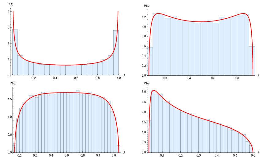
Having defined random POVMs, we then study their properties. We start with the spectrum of individual effect operators $A_i$. The behavior of their eigenvalues, in the large $d$ limit, is given by Voiculescu‘s free probability theory.

We also study the probability that two random POVMs $A$ and $B$ are compatible: is there another POVM $C$ with $k^2$ elements $C_{ij}$ such that the marginals of $C$ are $A_i = \sum_j C_{ij}$ and $B_j = \sum_i C_{ij}$ ? This question can be decided for concrete examples using semidefinite programming. However, in practice, when the size of the matrices becomes large, this technique can be computationally expensive. We then resort to compatibility and incompatibility criteria, which are simpler conditions that are only sufficient or only necessary for compatibility to hold (the situation is similar to the one in entanglement theory). We compare such compatibility criteria for generic POVMs, and we declare a winner! I will let you read the paper to find out which one that is. For incompatibility, the situation is more complicated: the known incompatibility criteria are very weak for random POVMs of large dimension with few outcomes. It is an open problem to invent new such criteria which can be insightful in this asymptotic regime.